Kinetics of Large Distributed Clusters

Summary

1. Martin Kleppmann's fatal mistake.
2. Physicochemical kinetics does mathematics.
3. The half-life of the cluster.
4. We solve nonlinear differential equations without solving them.
5. Nodes as a catalyst.
6. The predictive power of graphs.
7. 100 million years.
8. Synergy.

In the previous article, we discussed in detail Brewer's article and Brewer's theorem. This time we will analyze the post of Martin Kleppmann "The probability of data loss in large clusters".

In the mentioned post, the author attempts to simulate the following task. To ensure the preservation of data, the data replication method is usually used. In this case, in fact, it does not matter whether erasure is used or not. In the original post, the author sets the probability of dropping one node, and then raises the question: what is the probability of data loss when the number of nodes increases?

The answer is shown in this picture:

That is, the data loss grows proportional to the number of nodes.

Why does it matter? If we look at the size of the current clusters, we will see that their number has grown steadily over time. And so there's a reasonable question: Is it worth worrying about protecting your data and raising the replication factor? This has a direct impact on business, cost of ownership, and so on. Also, this example can be a great demonstration of how to produce a mathematically correct but incorrect result.

Cluster Modeling

It is useful to understand the model and simulation to demonstrate mistakes in calculations. If the model does not properly describe the actual behavior of the system, no matter what correct formulas are used, we can easily get the wrong result. And all because our model may not take into account any important parameters of the system that cannot be ignored. The science is to understand what's important and what is not.

To describe the life of the cluster, it is important to consider the dynamics of change and the relationship between different processes. This is the weak part of the original article because it has a static picture in it without any particular features associated with replication.

To describe the dynamics, I will use the methods of chemical kinetics, where I will use the ensemble of nodes instead of the particle ensemble. As far as I know, no one's used that formalism to describe the cluster behavior. So I'm going to improvise.

I introduce the following notation:

1. $N$ is the total number of cluster nodes.
2. $A$ is the number of operable nodes.
3. $F$ is the number of failed nodes.

Then it is obvious that:

$N = A + F$

The failed nodes include any problems: the disk got stuck, the processor, network, etc. broke down. I do not care about the reason, the very fact of the failure and inaccessibility of the data is important. In the future, of course, you can take into account more subtle dynamics.

Now let's write the kinetic equations of the processes of breaking and restoring cluster nodes:

$\\begin{aligned} A & \\rightarrow F,~k\_f &(1.1) \\\\ F & \\rightarrow A,~k\_a &(1.2) \\\\ \\end{aligned}$

These simplest equations mean the following. The first equation describes the process of node failure. It does not depend on any parameters and describes the isolated output of the node failure. Other nodes are not involved in this process. On the left, the original "composition" of the process participants is used, and the process products are on the right. Rate constants $k_f$ and $k_a$ specify the rate characteristics of processes for the failure and recovery of nodes, respectively.

Let us clarify the physical meaning of the rate constants. To do this, we write the kinetic equations:

$\\begin{aligned} \\frac{dA}{dt} &= -k\_f A + k\_a F \\\\ \\\\ \\frac{dF}{dt} &= k\_f A - k\_a F \\\\ \\end{aligned}$

From these equations we understand the meaning of constants $k_f$ and $k_a$. Assuming that there are no SREs and the cluster does not heal itself (i.e. $k_a = 0$), we immediately obtain the equation:

$\\begin{aligned} \\frac{dA}{dt} = -k\_f A \\\\ \\end{aligned}$

Or

$\\begin{aligned} A = N e^{-k\_f t} \\\\ \\end{aligned}$

That is, the quantity $1 / k_f$ is the half-life of the cluster for spare parts with the accuracy of $e / 2$. Let $\tau_f$ be the typical time of the transition of a single node from the state $A$ into the state $F$, and $\tau_a$ is the typical time of the transition of a single node from the state $F$ into the state $A$. Then

$\\begin{aligned} \\tau\_f &\\sim \\frac{1}{k\_f} \\\\ \\\\ \\tau\_a &\\sim \\frac{1}{k\_a} \\\\ \\\\ \\frac{\\tau\_a}{\\tau\_f} &= \\frac{k\_f}{k\_a} \\\\ \\end{aligned}$

Let's solve our kinetic equations. I want to make it right that I will cut corners wherever it is possible to get the simplest analytical dependencies that I will use for possible predictions and tuning.

Because my article reaches the maximum limit on the number of solutions of the differential equations, I will solve these equations using the steady state approximation:

$\\begin{aligned} \\frac{dA}{dt} = 0 \\Rightarrow F = A \\frac{k\_f}{k\_a} \\\\ \\end{aligned}$

Given that $F \ll N$ (this is a reasonable assumption, otherwise you need to buy better hardware or more advanced SREs), we get:

$\\begin{aligned} A &\\simeq N \\\\ F &= N \\frac{k\_f}{k\_a} \\\\ \\end{aligned}$

If we assume that the recovery time $\tau_a$ is approximately 1 week, and the time of death $\tau_f$ is approximately 1 year, we get that the ratio of broken nodes $p_f$ is:

$\\begin{aligned} p\_f = \\frac{F}{N} = \\frac{\\tau\_a}{\\tau\_f} \\approx 2\\% \\\\ \\end{aligned}$

Chunks

Let $U$ be the number of under-replicated chunks that need to be replicated after the nodes were failed when it goes into state $F$. Then to take chunks into account we improve our equations:

$\\begin{aligned} A & \\rightarrow F + U,~k\_f &(2.1) \\\\ F & \\rightarrow A,~k\_a &(2.2) \\\\ U + A & \\rightarrow H + A,~k\_r &(2.3) \\\\ \\end{aligned}$

Where $k_r$ is a replication rate constant of the process of the second order, and $H$ is a healthy chunk that dissolves in the total number of chunks.

The third equation should be clarified. It describes the second order process, not the first one:

$\\begin{aligned} U & \\rightarrow H,~k\_r \\\\ \\end{aligned}$

If we did that, we'd have a curve of Kleppmann, which is not part of my plan. In fact, all nodes are involved in the recovery process, and the more nodes we have, the faster replication process goes. This is due to the fact that the chunks from the failed nodes are distributed approximately evenly across the cluster so that each node spends $A$ times less time to replicate the under-replicated chunks. This means that the resulting chunks recovery rate from the failed nodes will be proportional to the number of available nodes $A$.

It is also worth noting that the equation (3) on the left and right are placed the same "substance" $A$, and it is not consumed or generated. The chemists would have stated immediately that $A$ is a catalyst in this case. And if you think carefully, it really is.

The steady state approach instantly provides the result:

$\\begin{aligned} \\frac{dU}{dt} = 0 = k\_f A - k\_r U A \\\\ \\end{aligned}$

or

$\\begin{aligned} U = \\frac{k\_f}{k\_r} \\\\ \\end{aligned}$

Amazing result! That is, the number of chunks to be replicated is independent of the number of nodes! This is due to the fact that increasing the number of nodes increases the resulting process rate (3), thus compensating the increased number of $F$ nodes. Catalysis!

Let's estimate this value. $\tau_r$ is the time of chunks recovery as if we had the only node. The node needs to replicate the 5 TB of the data, but the replication stream in bytes is 50 MB/s, then:

$\\begin{aligned} U = \\frac{\\tau\_r}{\\tau\_f} \\approx \\frac{1 \\times 10^5}{3.2 \\times 10^7} \\approx 3 \\times 10^{-3} \\\\ \\end{aligned}$

That is, $U \ll 1$ and you don't have to be afraid of data loss. It is worth taking into account that the loss of one chunk of three does not result in data loss.

Replication Planning

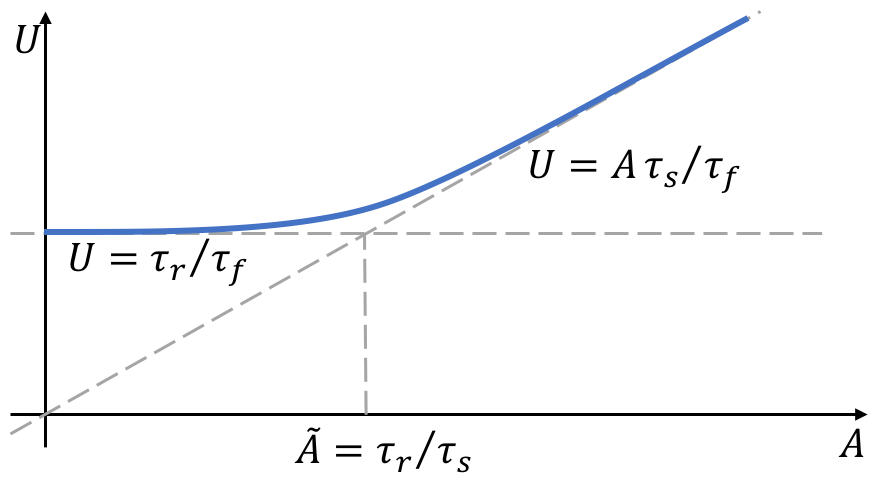
In the previous calculation, we made an implicit assumption that nodes instantly know about the specific chunks to be replicated, and immediately begins the replication. In reality, this is completely wrong: metadata servers need to understand that node goes away, then to understand the specific chunks to be replicated and start the replication process on the nodes. This is not instantaneous and takes a while, $\tau_s$, scheduling time.

To take advantage of the lag, I will use the theory of a transition state or an activated complex, which describes the process of moving through a saddle point on a multidimensional surface of potential energy. In our view, we will have some additional intermediate status $U^*$, which means that this chunk has been scheduled for replication, but the replication process has not started yet. That is, the next nanosecond replication will begin, but not picosecond earlier. Then our process system will take the final form:

$\\begin{aligned} A & \\rightarrow F + U,~k\_f &(3.1) \\\\ F & \\rightarrow A,~k\_a &(3.2) \\\\ U & \\rightarrow U^\*,~k\_s &(3.3) \\\\ U^\* + A & \\rightarrow H + A,~k\_r &(3.4) \\\\ \\end{aligned}$

Solving it, we find that:

$\\begin{aligned} \\frac{dU}{dt} &= k\_f A - k\_s U \\\\ \\\\ \\frac{dU^\*}{dt} &= k\_s U - k\_r U^\* A \\\\ \\end{aligned}$

Using the steady state approach, we find:

$\\begin{aligned} U &= A \\frac{k\_f}{k\_s} \\\\ U^\* &= \\frac{k\_f}{k\_r} \\\\ U\_{sum} &= U + U^\* = \\frac{\\tau\_r}{\\tau\_f} \\bigg( 1 + \\frac{A}{\\tilde A} \\bigg) \\\\ \\end{aligned}$

where:

$\\begin{aligned} \\tilde{A} = \\frac{\\tau\_r}{\\tau\_s} \\\\ \\end{aligned}$

As you can see, the result is the same as the previous one, except for the multiplier $(1 + A/\tilde A)$. Let's consider 2 limiting cases:

1. $A \ll \tilde A$. In this case, all of the previous statements are preserved: the number of chunks is not dependent on the number of nodes, which means that it does not grow with the growth of the cluster.
2. $A \gg \tilde A$. In this case, $U_{sum} \simeq A \tau_s / \tau_f$ and grows linearly with the increase of the number of nodes.

To determine the case let's estimate $\tilde A$. $\tau_s$ is a typical cumulative time for detecting a under-replicated chunk and planning its replication. Crude evaluation (using the "finger-to-sky" technique) gives a value of 100 s. Thus:

$\\begin{aligned} \\tilde{A} = \\frac{1 \\times 10^5}{100} = 1000 \\\\ \\end{aligned}$

Thus, further expansion of the cluster beyond this number will increase the likelihood of loss of chunk under these circumstances.

What can be done to improve the situation? It would seem possible to improve the asymptotic behavior by shifting the boundary $\tilde A$ by increasing $\tau_r$, but this will only increase the value of $U_{sum}$ without any real improvement. The most appropriate way to do this is to decrease $\tau_s$, which is the time to make a decision to replicate a chunk because $\tau_f$ depends on the characteristics of the hardware, and the software tools cannot influence on that.

Discussion of the Limit Cases

The proposed model actually splits clusters into two camps.

The first camp consists of relatively small clusters with the number of nodes < 1000. In this case, the probability of obtaining a under-replicated chunk is described by a simple formula:

$\\begin{aligned} U = \\frac{\\tau\_r}{\\tau\_f} \\\\ \\end{aligned}$

To improve the situation, two approaches can be applied:

1. Improve the hardware, thereby increasing $\tau_f$.
2. Speedup replication by reducing $\tau_r$.

These methods are generally clear enough.

In the second camp, we have large and extra-large clusters with a number of nodes > 1000. Here, the dependency will be defined as follows:

$\\begin{aligned} U = A \\frac{\\tau\_s}{\\tau\_f} \\\\ \\end{aligned}$

That is, it will be proportional to the number of nodes, which means that the subsequent increase in the cluster will have a negative impact on the likelihood of the appearance of under-replicated chunks. However, you can significantly reduce negative effects by using the following approaches:

1. Continue to increase $\tau_f$.
2. Improve the detection of under-replicated chunks and subsequent replication scheduling, thereby reducing $\tau_s$.

The second approach is no longer obvious. It seems that there is no significant difference between 20 seconds and 100 seconds for the value $\tau_s$. However, this value significantly influences the probability of under-replicated chunks. It is also not obvious that a dependency on $\tau_r$ is missing, i.e. the speed of replication does not play a role. This is understandable in this model: with the increase in the number of nodes, this speed is only increasing, so the replication of chunk is beginning to be significantly influenced by the constant addition of the replication process to detect and plan replication.

It's worth to consider $\tau_f$ in detail. In addition to the direct contribution to the chunks lifecycle, an increase of $tau_f$ has a positive effect on the number of available nodes, because:

$\\begin{aligned} A = N - F \\simeq N \\bigg( 1 - \\frac{\\tau\_a}{\\tau\_f} \\bigg) \\\\ \\end{aligned}$

That is, it increases the number of available nodes. So, an improvement of $\tau_f$ directly affects the availability of the cluster resources, speeding up the computation, while increasing the reliability of the data storage. On the other hand, the improvement in hardware quality directly affects the cost of ownership of the cluster. The model provides a quantitative measure of the economic feasibility of this type of solution.

Comparison of Approaches

I would like to compare the two approaches. The following graphs will tell you this eloquently.

You can only see a linear dependency from the first graph, but it will not answer the question: "What do you need to do to improve the situation?" The second picture describes a more complex model that can immediately provide answers to questions about what to do and how to improve the behavior of the replication process. Moreover, it provides a recipe for a quick way, literally in mind, estimating the effects of some architectural decisions. In other words, the predictive strength of the developed model is at a qualitatively different level.

Chunk Loss

Now let's obtain the typical time of chunk loss. To do this, we write out the kinetics of the processes of formation of such chunks taking into account the replication factor 3:

$\\begin{aligned} A & \\rightarrow F + U,~k\_f &(4.1) \\\\ F & \\rightarrow A,~k\_a &(4.2) \\\\ U & \\rightarrow U^\*,~k\_s &(4.3) \\\\ U^\* + A & \\rightarrow H + A,~k\_r &(4.4) \\\\ U & \\rightarrow F + U\_2,~k\_f &(4.5) \\\\ U^\* & \\rightarrow F + U\_2,~k\_f &(4.6) \\\\ U\_2 & \\rightarrow U\_2^\*,~k\_s &(4.7) \\\\ U\_2^\* + A & \\rightarrow U + A,~k\_r &(4.8) \\\\ U\_2 & \\rightarrow F + L,~k\_f &(4.9) \\\\ U\_2^\* & \\rightarrow F + L,~k\_f &(4.10) \\\\ \\end{aligned}$

Here $U_2$ indicates the number of under-replicated chunks that lost two copies, $U_2^*$ is an intermediate state, similar to $U^*$ corresponding to substance $U_2$, and $L$ is the lost chunk. Then:

$\\begin{aligned} \\frac{dL}{dt} &= k\_f \\big( U\_2 + U\_2^\* \\big) \\\\ \\tau\_l &= \\frac{1}{k\_f \\big( U\_2 + U\_2^\* \\big) } \\\\ \\end{aligned}$

Where $\tau_l$ is the typical time of the formation of the lost chunk. We'll solve our system for two limit cases when $A = 1000$.

$A \ll \tilde A$, then

$\\begin{aligned} \\tau\_l = A \\frac{\\tau\_f^3}{\\tau\_r^2} \\approx 100\\ 000\\ 000\\ years \\\\ \\end{aligned}$

For the case $A \gg \tilde A$ we obtain:

$\\begin{aligned} \\tau\_l = \\frac{\\tau\_f^3}{A \\tau\_s^2} \\approx 100\\ 000\\ 000\\ years \\\\ \\end{aligned}$

That is, the typical time of the formation of the lost chunk is 100 million years! There are roughly similar values for the mentioned two cases as we are in the transition zone. The typical time value $\tau_l$ tells for itself and everyone can draw conclusions by itself.

It is worth mentioning one thing, however. In the case $A \ll \tilde A$ the value $U$ is a constant and does not depend on $A$. But in an expression for $\tau_l$ we obtain a reciprocal dependency, that is, as the cluster grows, triple replication even improves data safety! And finally, as the cluster continues to grow, the situation changes exactly to the opposite.

Conclusion

The article consistently introduces an innovative way of simulating the kinetics of large cluster processes. The approximate model for describing the dynamics of a cluster can be considered as probabilistic characteristics that describe the data loss.

Of course, this model is only the first approximation to what is actually happening on the cluster. Here we have only taken into account the most important processes in order to produce a qualitative result. But even such a model allows you to judge what is happening within the cluster and also provides recommendations to improve the situation.

However, the suggested approach allows for more accurate and reliable results based on a subtle consideration of different factors and an analysis of the actual performance of the cluster. Below is a far from the exhaustive list for improving the model:

1. Cluster nodes can fail due to various hardware failures. The failure of a particular node usually has a different probability. Moreover, a failure, for example, of a processor, does not lose data, but only gives a temporary inaccessibility of the node. It is easy to take into account in the model, introducing different states $F_{proc}$, $F_{disk}$, $F_{mem}$ etc, with different process rates and different consequences.
2. Not all nodes are equally useful. Different batches may have different natures and frequency of failures. This can be taken into account in the model by introducing $A_1$, $A_2$, and so on, at different rates of the corresponding processes.
3. The addition of different types of nodes to the model: partially damaged discs, banned, etc. For example, you can analyze the impact of shutting down a rack and determining the typical speeds of a cluster's transition to a steady mode. In doing so, the dynamics of chunks and nodes can be visualized by numerically solving differential equations.
4. Each storage disk has slightly different read/write characteristics, including latency and bandwidth. However, you can estimate more accurately the rate constants of the processes by integrating the corresponding disk-specific distribution functions by analogy with the velocity constants in the gases, which are integrated over Maxwell–Boltzmann distribution.

Thus, on the one hand, the kinetic approach allows simplify the description and analysis, and on the other hand, has a very serious potential for introducing additional subtle factors and processes based on the analysis of cluster working data, adding specific details on demand. You can evaluate the impact of each factor's contribution to the resulting equations, allowing you to simulate improvements to make them useful. In the simplest case, this model enables you to quickly get analytical dependencies by providing recipes to improve the situation. The simulation can be bi-directional in nature: You can iteratively improve the model by adding processes to the kinetic equation system and try to analyze the potential system improvements by entering processes in the model. That is, to simulate improvements before the expensive changes by direct implementing them in your code and hardware.

In addition, it is always possible to move to numerical integration of stiff nonlinear differential equations obtaining the dynamic of the system and response to specific effects or small perturbations.

Thus, a synergy of seemingly unrelated fields of knowledge can produce astonishing results with indisputable predictive power.

References

[1] Cap Theorem Myths.
[2] Spanner, TrueTime and the CAP Theorem.
[3] The probability of data loss in large clusters.
[4] Chemical kinetics.
[5] Activated complex.
[6] Steady state approximation.
[7] Maxwell–Boltzmann distribution.